apples <- 10
oranges <- 6
durians <- 2

fruit_n <- sum(apples, oranges, durians)
cat("We have in total", fruit_n, "fruits.")
We have in total 18 fruits.RStudio and R scripts
Last week you started your R journey with the R Console.
Working with the R Console can quickly become a bit inefficient: imagine having to run a lot of code, read a lot of different files, keeping track of a lot of variables and so on…
This is what Integrated Development Environment (IDE) software comes in: an IDE is just a graphical interface to programming languages that offer users with a lot of features to help them streamline their workflow. (But don’t get fooled! You still have to learn how to code.)
R has a dedicated IDE called RStudio. This is what we will use from this week on. Note that RStudio even works with Python and many other languages!
Beginners usually have trouble understanding the difference between R and RStudio.
Let’s use a car analogy.
What makes the car go is the engine and you can control the engine through the dashboard.
You can think of R as an engine and RStudio as the dashboard.
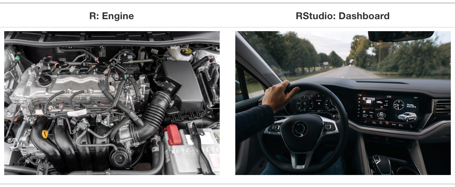
R is a programming language.
We use programming languages to interact with computers.
You run commands written in a console and the related task is executed.
RStudio is an Integrated Development Environment or IDE.
It helps you using R more efficiently.
It has a graphical user interface or GUI.
The next section will give you a tour of RStudio.
When you open RStudio, you can see the window is divided into 3 panels:
Blue (left): the R Console. This is basically the same thing as the R Console you have been using last week.
Green (top-right): the Environment tab.
Purple (bottom-right): the Files tab.
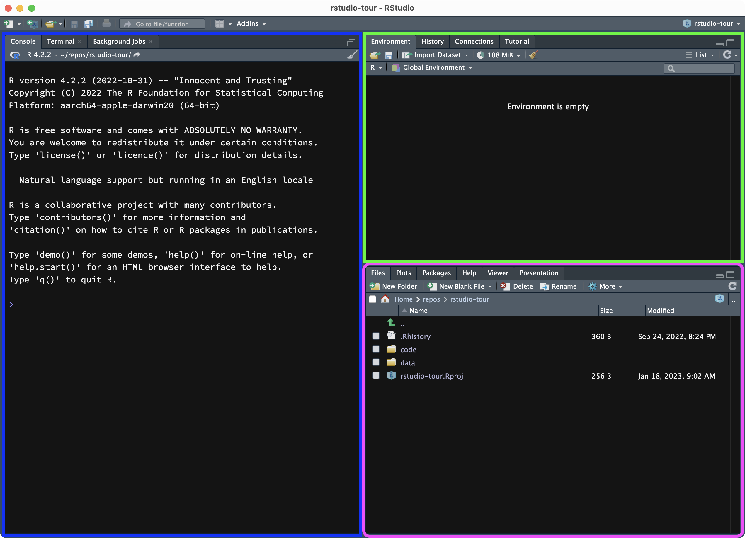
The Console is where R commands can be executed.
The Environment tab lists the objects created with R, while in the Files tab you can navigate folders on your computer to get to files and open them in the file Editor.
RStudio is an IDE (see above) which allows you to work efficiently with R, all in one place.
Note that files and data live in folders on your computer, outside of RStudio: do not think of RStudio as an app where you can save files in.
All the files that you see in the Files tab are files on your computer and you can access them from the Finder or File Explorer as you would with any other file.
In principle, you can open RStudio and then navigate to any folder or file on your computer.
However, there is a more efficient way of working with RStudio: RStudio Projects.
An RStudio Project is a folder on your computer that has an .Rproj file.
A special type of RStudio project are Quarto Projects. We will use these in this course.
A Quarto Project is an RStudio project which has a _quarto.yml file.
You will learn a bit more about the _quarto.yml file below.
You can create as many Quarto Projects as you wish, and I recommend to create one per project (your dissertation, a research project, a course, etc…). Also, I strongly recommend that you DO NOT save projects on One Drive, but do back up your files there (or at least somewhere else). This is known to cause issues, so it is best to save projects on your Documents folder, for example.
We will create a Quarto Project for this course (meaning, you will create a folder for the course which will be the Quarto Project). You will have to use this project/folder throughout the semester.
To create a new Quarto Project, click on the button that looks like a transparent light blue box with a plus, in the top-left corner of RStudio. A window like the one below will pop up.
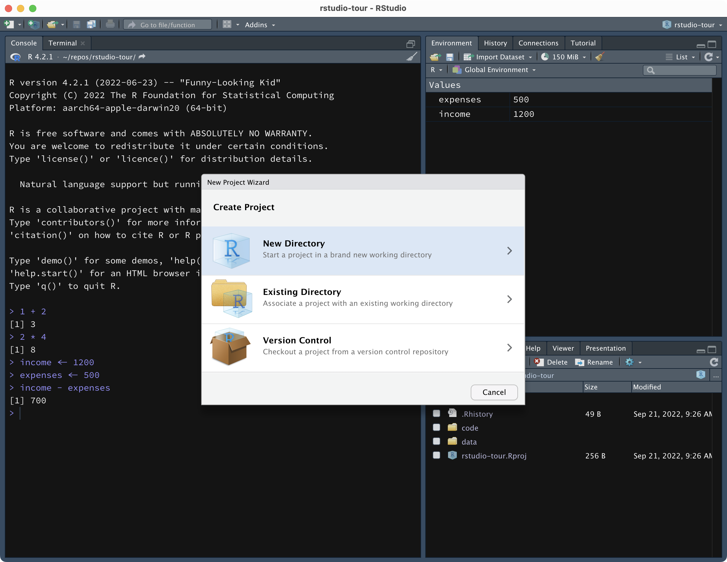
Click on New Directory then Quarto Project.
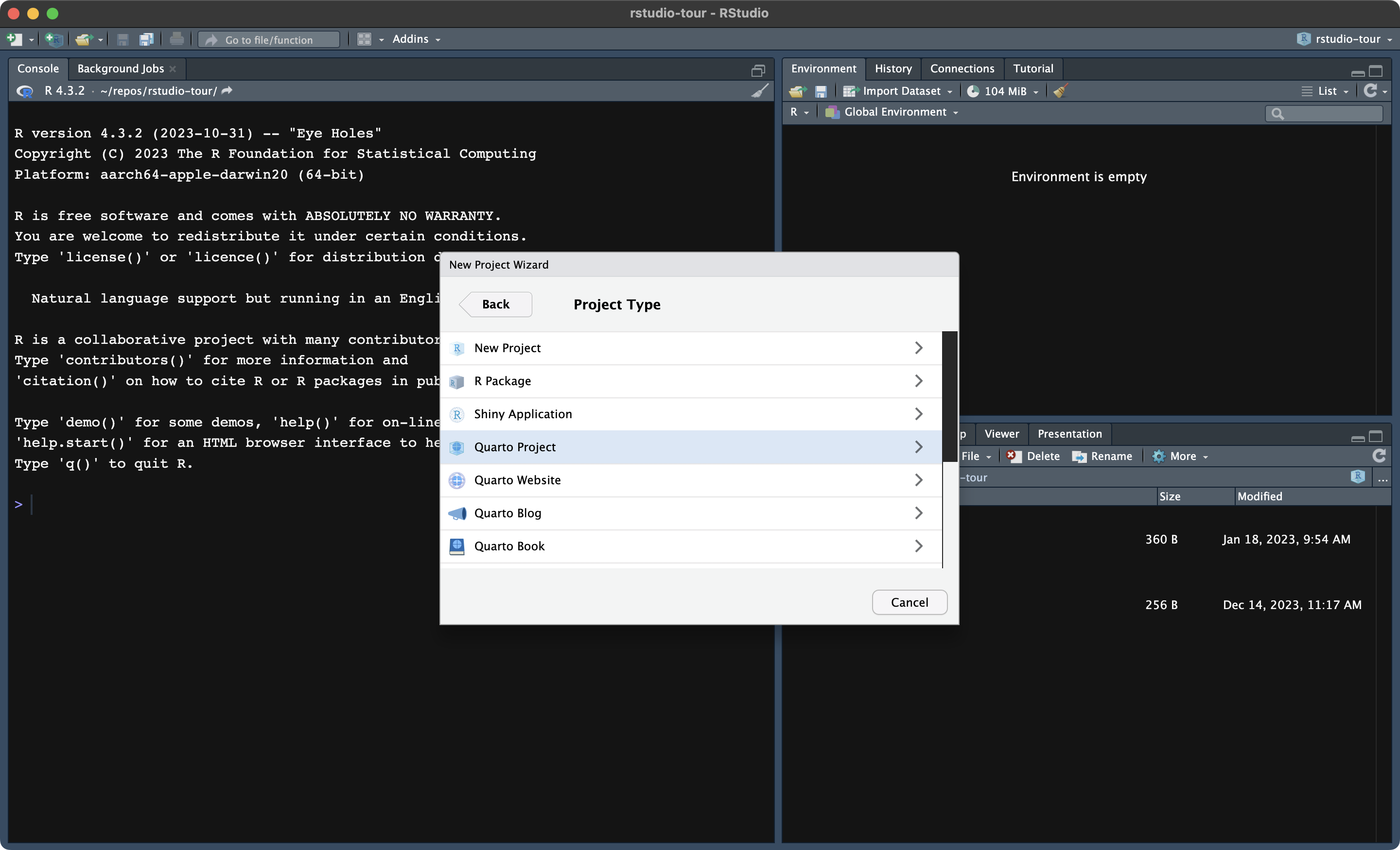
Now, this will create a new folder (aka directory) on your computer and will make that an RStudio Project (meaning, it will add a file with the .Rproj extension to the folder; the name of the file will be the name of the project/folder).
Give a name to your new project, something like the name of the course and year (e.g. dal-2024).
Then you need to specify where to create this new folder/Project. Click on Browse… and navigate to the folder you want to create the new folder/Project in. DO NOT use One Drive, as mentioned above.
**Make sure to untick the Use visual markdown editor option and that the engine is set to knitr.** The settings should be exactly as shown below.
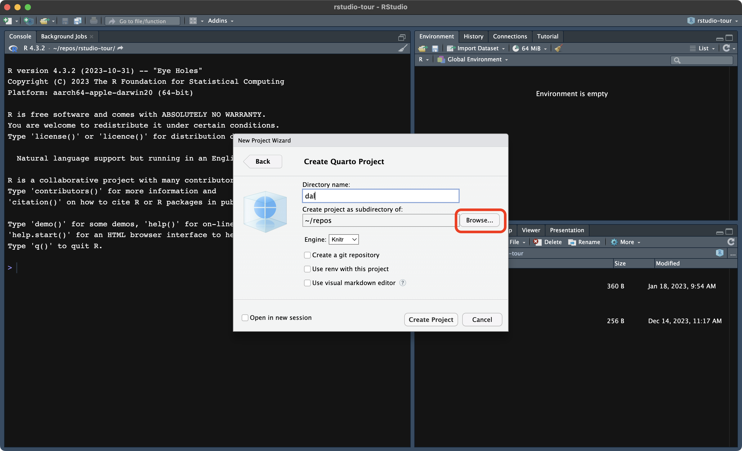
When done, click on Create Project. RStudio will automatically open your new project. A .qmd file will be opened automatically: you can safely close that for now.
The project folder will contain the following files:
A _quarto.yml file, that tells RStudio this is a Quarto Project.
A .qmd file, named after the name of project. You will learn about .qmd files next week. You can close this file if it is still open in the File panel.
An .rproj file, named after the name of the project. This file is there just to inform RStudio that this folder is a project and you are not supposed to edit it.
When working through these tutorials, always make sure you are in the course’s RStudio Quarto Project you created.
You know you are in an RStudio Project because you can see the name of the Project in the top-right corner of RStudio, next to the light blue cube icon.
If you see Project (none) in the top-right corner, that means your are not in an RStudio Project.
To make sure you are in the RStudio project, to open the project go to the project folder in File Explorer or Finder and double click on the .Rproj file.
There are several ways of opening an RStudio Project:
You can go to the RStudio Project folder in Finder or File Explorer and double click on the .Rproj file.
You can click on File > Open Project in the RStudio menu.
You can click on the project name in the top-right corner of RStudio, which will bring up a list of projects. Click on the desired project to open it.
Before moving on, there are a few important settings that you need to change. See figure below for how they should look.
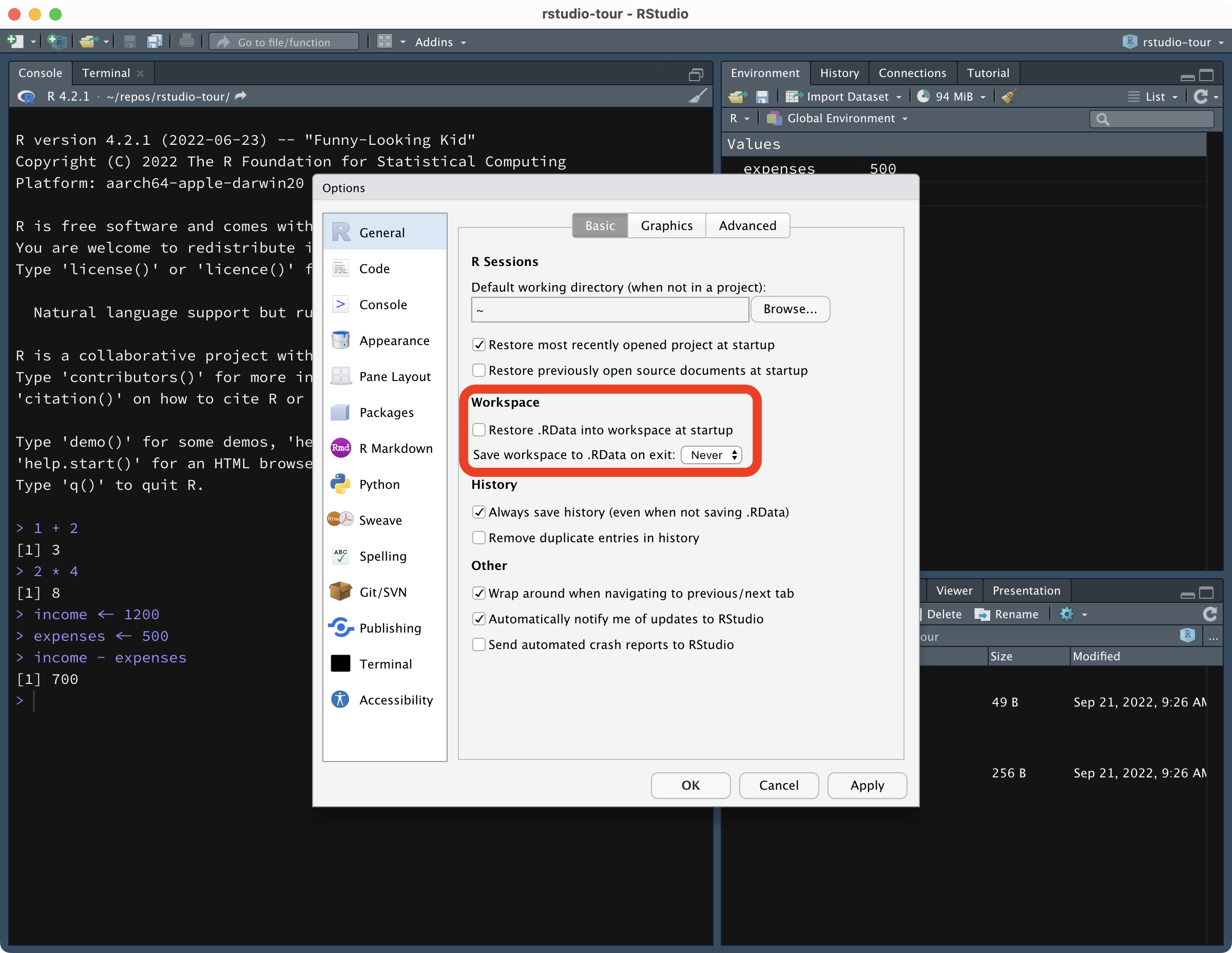
Open the RStudio preferences (Tools > Global options..., might be different on Windows).
Un-tick Restore .RData into workspace at startup.
Select Never in Save workspace to .RData on exit.
Click OK to confirm the changes.
True or false?
RStudio executes the code.
R is a programming language.
An IDE is necessary to run R.
RStudio projects are folders with an .Rproj file.
The project name is shown in the top-right corner of RStudio.
Now you can run R code in the Console from within RStudio.
Try the following:
apples <- 10
oranges <- 6
durians <- 2
fruit_n <- sum(apples, oranges, durians)
cat("We have in total", fruit_n, "fruits.")We have in total 18 fruits.The sentence We have in total 18 fruits. will be printed on the Console.
Moreover, you will see that the variables we created (apples, oranges, durians, fruit_n) are listed in the Environment tab in the top-right panel of RStudio.
This is much better than having to use ls() to remember which variables you have created.
Now create three more variables:
They should all be vectors of at least three elements.
You should create one numeric, one character and one logical vector.
To create vectors, you should use the c() function.
Now check the Environment tab: your new variables will be there. The values of each variable should be prefixed with:
The vector type: num for numeric, chr for character and logi for logical.
And the length of the vector in the form [1:N] where N is the number of element/values in the vector.
That’s neat! You can obtain the length of a vector (i.e. the number of element/values) with the length() function.
The length of a vector is the number of values contained in the vector.
You can obtain the vector length with length().
For example:
Remember you can always check the type of vector with the class() function.
So far, you’ve been asked to write code in the Console and run it there.
But this is not very efficient. Every time, you need to write the code and execute it in the right order and it quickly becomes very difficult to keep track of everything when things start getting more involved.
A solution is to use R scripts.
An R script is a file with the .R extension that contains R code.
For the rest of this tutorial, you will write all code in an R script.
First, create a folder called code in your project folder. You can do so from within RStudio, in the Files tab or you can just create the folder in the File Explorer/Finder. This will be the folder where you will save all of your R scripts and other code files.
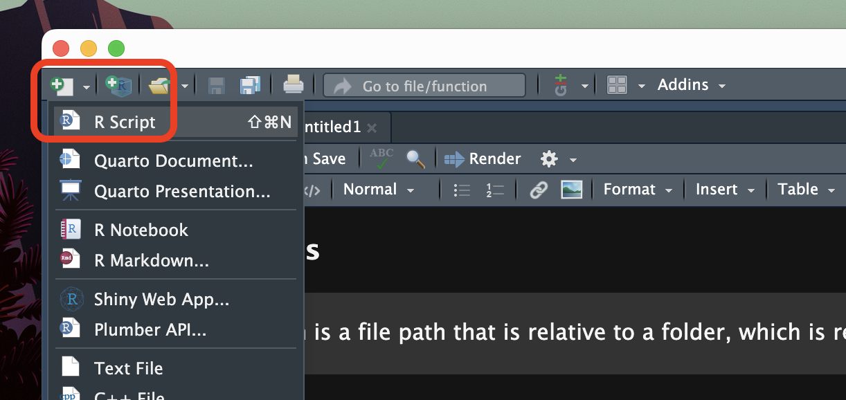
Now, to create a new R script, look at the top-left corner of RStudio: the first button to the left looks like a white sheet with a green plus sign. This is the New file button. Click on that and you will see a few options to create a new file.
Click on R Script. A new empty R script will be created and will open in the File Editor window of RStudio.
Note that creating an R script does not automatically saves it on your computer. To do so, either use the keyboard short-cut CMD+S/CTRL+S or click on the floppy disk icon in the menu below the file tab.
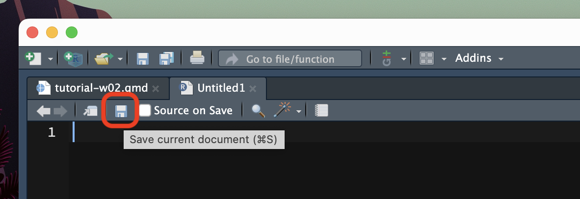
Save the file inside the code/ folder with the following name: tutorial-w02.R.
Remember that all the files of your RStudio project don’t live inside RStudio but on your computer.
So you can always access them from the Finder or File Explorer! However, do not open a file by double clicking on it from the Finder/File Explorer.
Rather, open the RStudio project by double clicking on the .Rproj file and then open files from RStudio to ensure you are working within the RStudio project and the working directory is set correctly.
Now your script is ready to be filled with code. Copy the following lines of code and paste them at the top of your R script (this is the same code as above).
Now, there are several ways to run code.
One is to click on the Run button. You can find this in the top-right corner of the script window.

When you click Run, R runs the line of code that currently has the text cursor (|) and then moves the cursor to the next line (you can click Run again to run the line and so on.) You can also select multiple lines on the script and click Run, and all the selected lines will be run.
An alternative way is to place the text cursor on the line of code you want to run and then press CMD+ENTER/CTRL+ENTER. This will run the line of code and move the text cursor to the next line of code, as if you had clicked Run.
You can even select multiple lines of code (as you would select text) and press CMD+ENTER/CTRL+ENTER to run multiple lines of code!
Now that you know how to use R scripts and run code in them, I will assume that you will keep writing new code from this tutorial in your script and run it from there!
In the next section, you will learn how to extend R capabilities with packages.
When you install R, a library of packages is also installed. Packages provide R with extra functionalities, usually by making extra functions available for use. You can think of packages as “plug-ins” that you install once and then you can “activate” them when you need them. The library installed with R contains a set of packages that are collectively known as the base R packages, but you can install more any time!
Note that the R library is a folder on your computer. Packages are not installed inside RStudio. Remember that RStudio is just an interface.
You can check all of the currently installed packages in the bottom-right panel of RStudio, in the Packages tab. There you can also install new packages.
The R library contains the base R packages and all the user-installed packages.
R packages provide R with extra functionalities and are installed into the R library.
If you want to find the path of the R library on your computer, type .libPaths() in the Console. The function returns (i.e. outputs) the path or paths where your R library is.
You can install extra packages in the R library in two ways:
install.packages() function. This function takes the name of the package you want to install as a string, for example install.packages("cowsay").If you install a package with the function install.packages(), do so in the Console! Do not include this function in your scripts (this is because you install packages only once, see below)).
Packages tab in the bottom-right panel of RStudio and click on Install. A small window will pop up. See the screenshot below.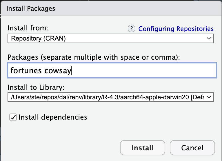
Go ahead and try to install a package using the second method. Install the cowsay and the fortunes packages (see picture above for how to write the packages). After installing you will see that the package fortunes is listed in the Packages tab.
To install packages, go to the Packages tab of the bottom-right panel of RStudio and click on Install.
In the “Install packages” window, list the package names and then click Install.
You need to install a package ONLY ONCE! Once installed, it’s there for ever, saved in the R library. You will be able to use all of your installed packages in any RStudio project you create.
Now, to use a package you need to attach the package to the current R session with the library() function. Attaching a package makes the functions that come with the package available to us.
You need to attach the packages you want to use once per R session.
Note that every time you open RStudio, a new R session is started.
Let’s attach the cowsay and fortunes packages. Write the following code at the top of your R script, before all the other code you wrote.
Note that library(cowsay) takes the name of the package without quotes, although if you put the name in quotes it also works. You need one library() function per package (there are other ways, but we will stick with this one).
Packages are attached with the library(pkg.name) function, where pkg.name is the name of the package.
It is customary to put all the packages used in the script at the top of the script.
Now you can use the functions provided by the attached packages. Try out the say() function from the cowsay package.
Write the following in your R script and run it!
(I know, the usefulness of the package might be questionable, but it is fun!)
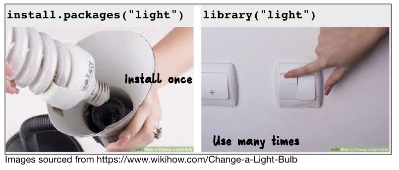
Remember, you need to install a package only once but you need to attach it with library() every time you start R.
Think of install.packages() as mounting a light bulb (installing the package) and library() as the light switch (attaching the package).
To learn what a function does, you can check its documentation by typing in the Console the function name preceded by a ? question mark. Type ?say in the Console and hit ENTER to see the function documentation. You should see something like this:
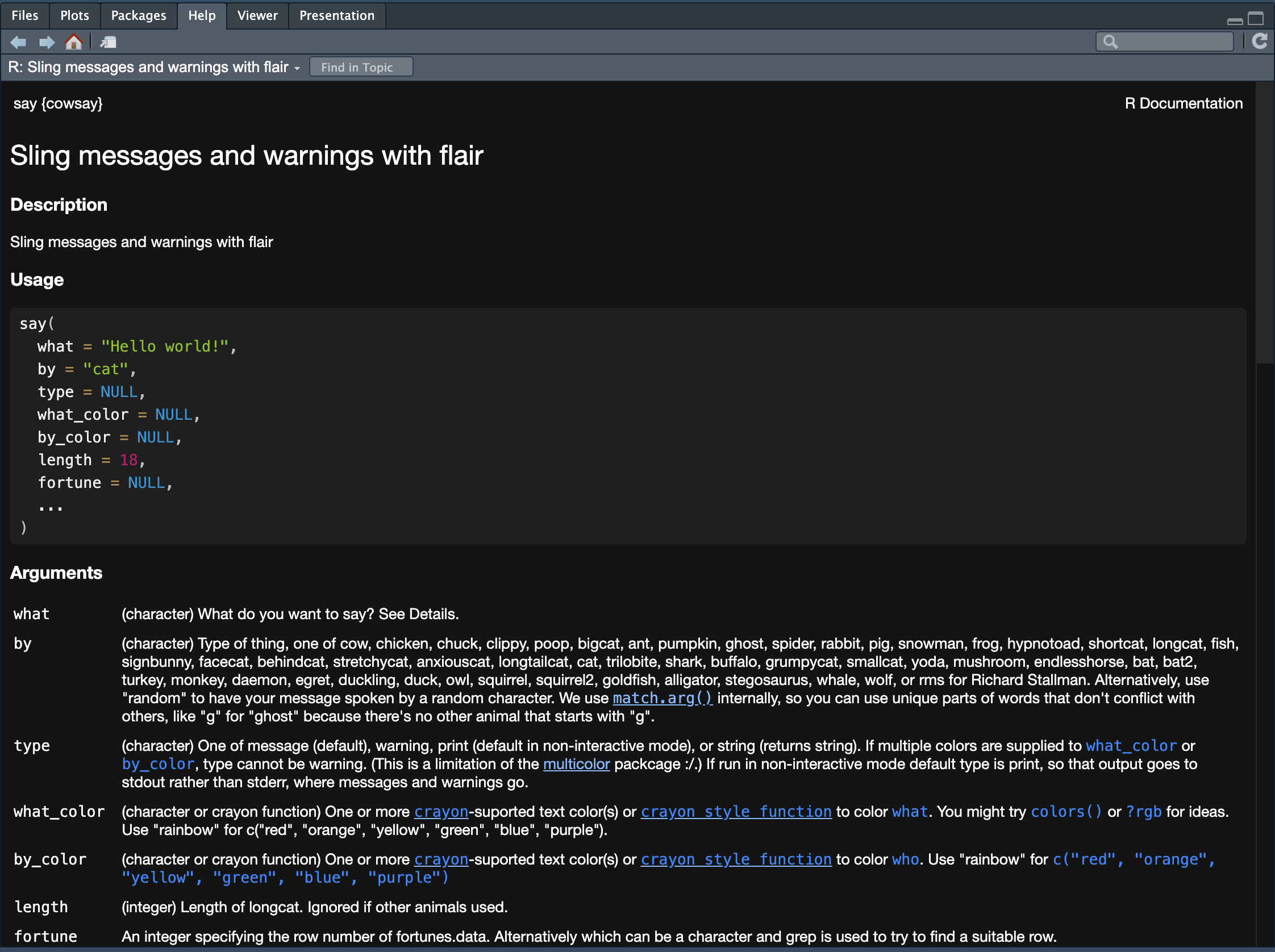
The Description section is usually a brief explanation of what the function does.
In the Usage section, the usage of the function is shown by showing which arguments the function has and which default values (if any) each argument has. When the argument does not have a default value, NULL is listed as the value.
The Arguments section gives a thorough explanation of each function argument. (Ignore … for now).
How many arguments does say() have? How many arguments have a default value?
Default argument values allow you to use the function without specifying those arguments. Just write say() in your script on a new line and run it. Does the output make sense based on the Usage section of the documentation?
The rest of the function documentation usually has further details, which are followed by Examples. It is always a good idea to look at the example and test them in the Console when learning new functions.
This was a question about terminology. In R, you attach packages from the library using (confusingly) the library() function.
Sometimes we might want to add a few lines of text in our script, for example to take notes.
You can add so-called comments in R scripts, simply by starting a line with #. If you add # at the end of a line, anything after that will be considered a comment. Comments are simply skipped when R runs code.
You can add text comments in R scripts by starting a new line with # or by writing text preceded by # at the end of any line of code.
For example:
[1] 9[1] 9You made it! You completed this week’s tutorial.
Here’s a summary of what you learnt.
R is a programming language while RStudio is an IDE.
Quarto projects are folders with an .Rproj file (you can see the name of the project you are currently in in the top-right corner of RStudio).
R scripts contain R code and help you keep track of the code you run.
R packages provide R with extra functionalities. The R library is a folder with all the installed packages.
.libPaths() returns the path(s) to the R library.
library() attaches R packages (i.e. makes the package’s functions available for use).
You can inspect the documentation of any function by running ?function in the Console (where function is the function’s name, e.g. ?paste).
You can write text comments in R scripts by starting a line with #.