QML - Week 6
Regression models: the basics
Word frequency and reaction times
What is the relationship between a word’s lexical frequency and reaction times in a lexical decision task in Croatian?
Data from Lexical decision times for nouns from the Croatian Psycholinguistic Database.
Lexical decision task (is it a real Croatian word?)
Reaction times.
Word frequency: counts from the Croatian web Corpus hrWaC.
Which relationship?
Reaction times
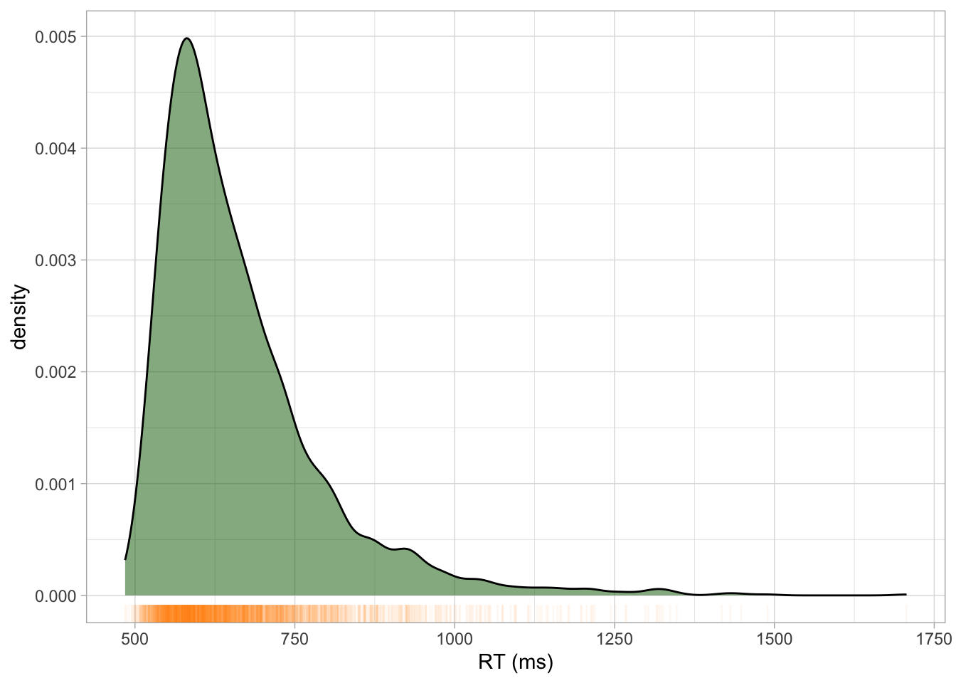
Word frequency and RTs
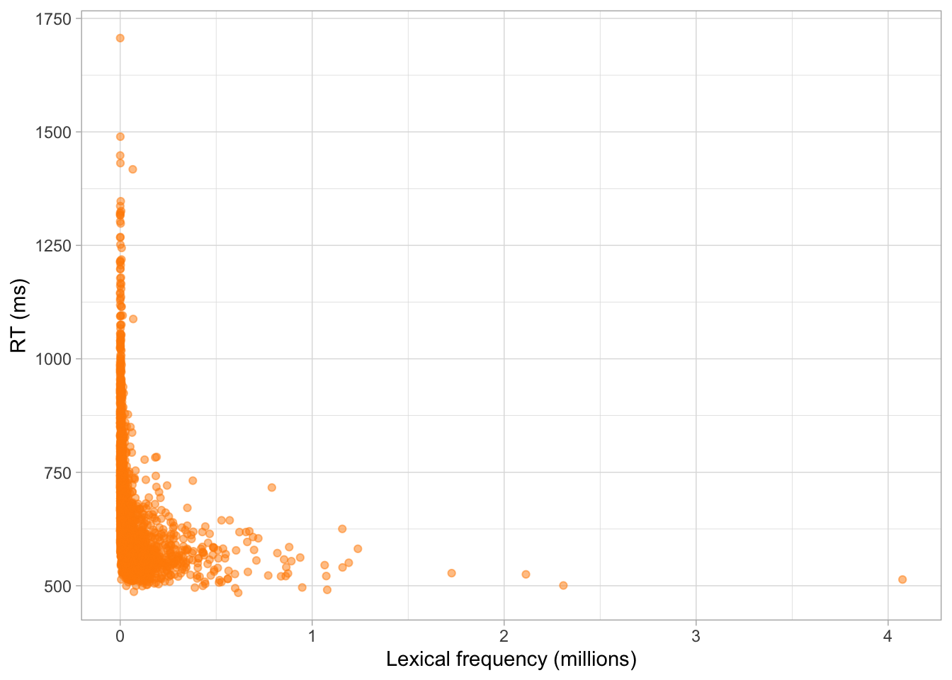
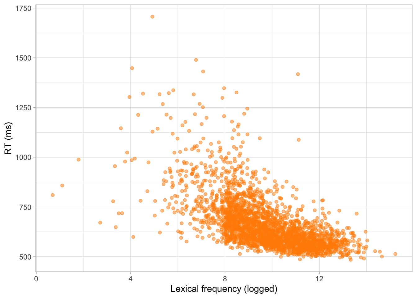
Logged word frequency and RTs
Gaussian model of RT
\[RT \sim Gaussian(\mu, \sigma)\]
But we want to know what happens to RTs depending on the value of lexical frequency…
Then we let the mean \(\mu\) vary by lexical frequency!
\[\begin{aligned} RT_i & \sim Gaussian(\mu_i, \sigma)\\ \mu_i & = \beta_0 + \beta_1 \cdot logf_i \end{aligned}\]
The equation of a line
\[y = \beta_0 + \beta_1 \cdot x\]
\(\beta_0\) is the line intercept: the \(y\) value when \(x\) is
0zero.\(\beta_1\) is the line slope: the change in \(y\) for each unit-increase of \(x\).
Regression model
\[\begin{aligned} RT_i & \sim Gaussian(\mu_i, \sigma)\\ \mu_i & = \beta_0 + \beta_1 \cdot logf_i & \text{[Regression equation]} \end{aligned}\]
A regression model is a model that uses the equation of a line (the regression equation).
The model estimates \(\beta_0\) (the intercept), \(\beta_1\) (the slope) and \(\sigma\) from the data (i.e. the observed \(RT\) and \(logf\) values).
\(\beta_0\), intercept
- Mean RT value when logged frequency is
0zero (i.e. when word frequency is 1;exp(0)= 1).
\(\beta_1\), slope
- Change in mean RT for each unit increase of log-frequency (when log-frequency goes from \(x\) to \(x + 1\)).
Fit model in brms
Model results
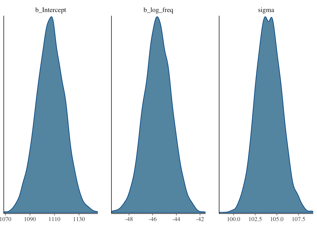
Posterior draws
# A draws_df: 1000 iterations, 4 chains, and 6 variables
   b_Intercept b_log_freq sigma Intercept lprior   lp__
1         1096        -44   107       664    -11 -15847
2         1120        -47   103       667    -11 -15846
3         1095        -45   105       660    -11 -15846
4         1121        -47   104       667    -11 -15845
5         1103        -45   102       663    -11 -15845
6         1105        -45   106       665    -11 -15845
7         1110        -46   103       664    -11 -15844
8         1092        -44   103       663    -11 -15845
9         1125        -47   103       666    -11 -15846
10        1114        -46   104       662    -11 -15845
# ... with 3990 more draws
# ... hidden reserved variables {'.chain', '.iteration', '.draw'}
Posterior of \(\beta_1\)
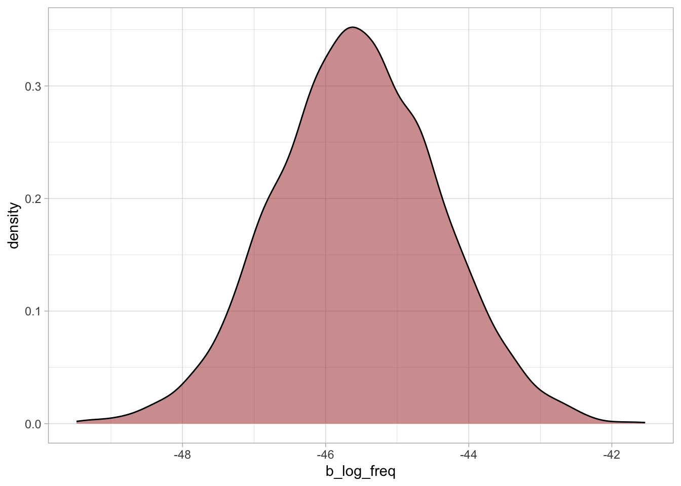
Posterior of \(\beta_1\) with CrIs
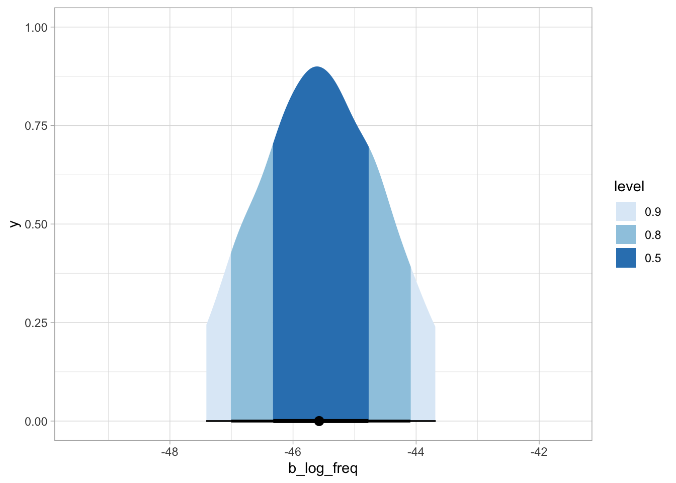
CrIs of \(\beta_1\)
Expected values
\[\begin{aligned} \mu_i & = \beta_0 + \beta_1 \cdot logf_i\\ \mu_{[logf = 4]} & = \beta_0 + \beta_1 \cdot 4\\ \mu_{[logf = 12]} & = \beta_0 + \beta_1 \cdot 12\\ \end{aligned}\]
Plotting expected values
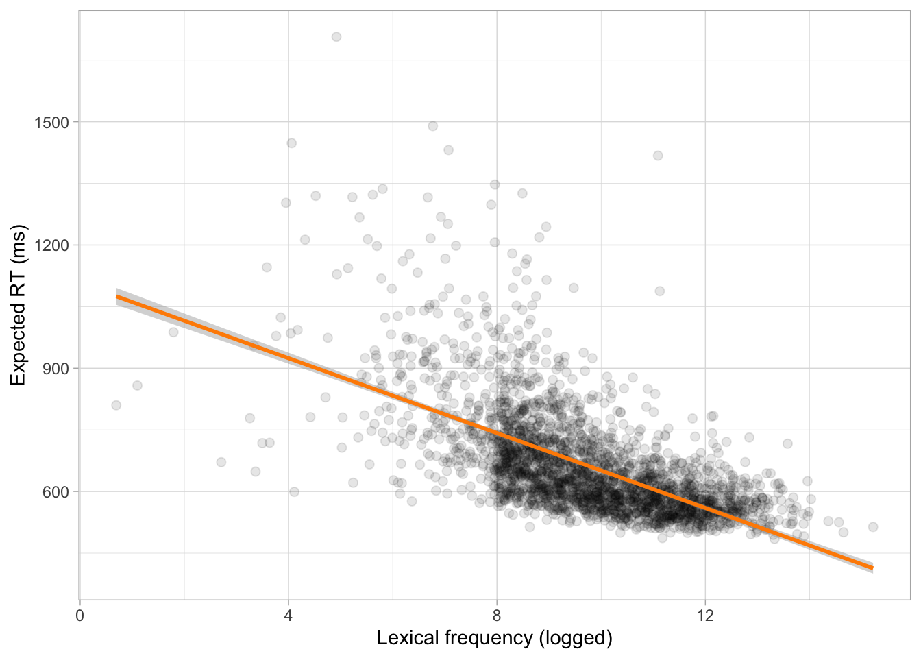
Word frequency and reaction times (bis)
What is the relationship between a word’s lexical frequency and reaction times in a lexical decision task in Croatian?
When log-frequency is 0, the mean RTs are between 1084 and 1129 ms at 95% confidence.
For each unit increase of log-frequency, the mean RTs decrease by 43-48 ms, at 95% confidence.
Correlation in NOT causation
Be careful!
Correlation between two variables: they co-vary, i.e. they show a systematic association (their values tend to vary together in a consistent pattern).
Spurious correlations: two variables can be correlated because of bias from another variable.
- Number of plant names in a language vs. biodiversity of the region
- Languages in biodiverse regions have more words for plants.
- Mediator: cultural reliance on plants.
- Language endangerment vs. economic development
- Higher economic development is associated with greater language endangerment.
- Confounder: colonial history.
- Language prestige vs government policy
- High prestige languages and officially supported languages each attract learners.
- Collider: If you only look at languages with many learners, prestige and policy might appear related even if they’re not causally connected.
But it is if you use causal inference…
Causal inference
Correlation can be interpreted causally if you adopt a causal inference approach.
Learn about it in McElreath’s textbook Statistical Rethinking. Also check STeW.