QML - Week 8

Bernoulli regression models

Stefano Coretta

Bouba and kiki

Holland and Wertheimer (1964), Chen et al. (2016)

Cross-modality

• There are links between the auditory and visual modalities.

• A lot of research this concept, in fact originated with Köhler (1929) who used “takete” and “maluma” (not the singer).

• Koppensteiner, Stephan, and Jäschke (2016) ask if not only shape, but also motion patterns enter in the cross-modality link.

Motion patterns

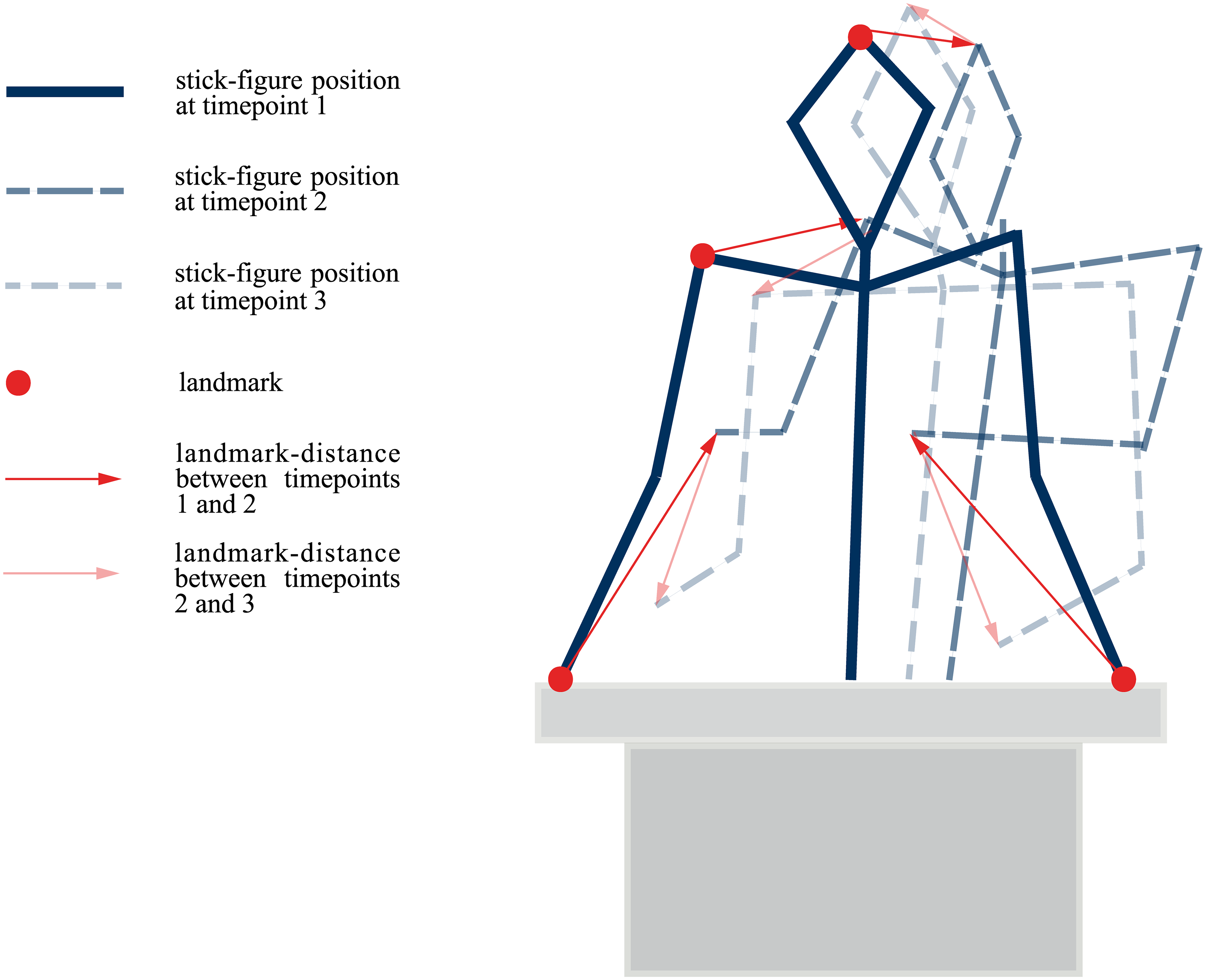
Koppensteiner, Stephan, and Jäschke (2016)

Motion patterns

Koppensteiner, Stephan, and Jäschke (2016)

• 46 students (24 females and 22 males; age M = 25.1 years, SD = 3.6) of the University of Vienna.

• They saw a word (takete or maluma) and two stick-figures moving.

• They had to pick the stick figure they thought was described by the word.

The data

kopper <- read_delim("data/koppensteiner2016/takete_maluma.txt")
kopper

# A tibble: 460 × 5
   Tak_Mal_Stim Answer  Corr_1_Wrong_0 Rater                   Female_0
   <chr>        <chr>            <dbl> <chr>                      <dbl>
 1 Takete       CORRECT              1 10MacI_12_10_11_59_.txt        0
 2 Takete       CORRECT              1 10MacI_12_10_11_59_.txt        0
 3 Takete       CORRECT              1 10MacI_12_10_11_59_.txt        0
 4 Takete       CORRECT              1 10MacI_12_10_11_59_.txt        0
 5 Takete       CORRECT              1 10MacI_12_10_11_59_.txt        0
 6 Maluma       CORRECT              1 10MacI_12_10_11_59_.txt        0
 7 Takete       CORRECT              1 10MacI_12_10_11_59_.txt        0
 8 Takete       CORRECT              1 10MacI_12_10_11_59_.txt        0
 9 Maluma       CORRECT              1 10MacI_12_10_11_59_.txt        0
10 Takete       CORRECT              1 10MacI_12_10_11_59_.txt        0
# ℹ 450 more rows

Accuracy

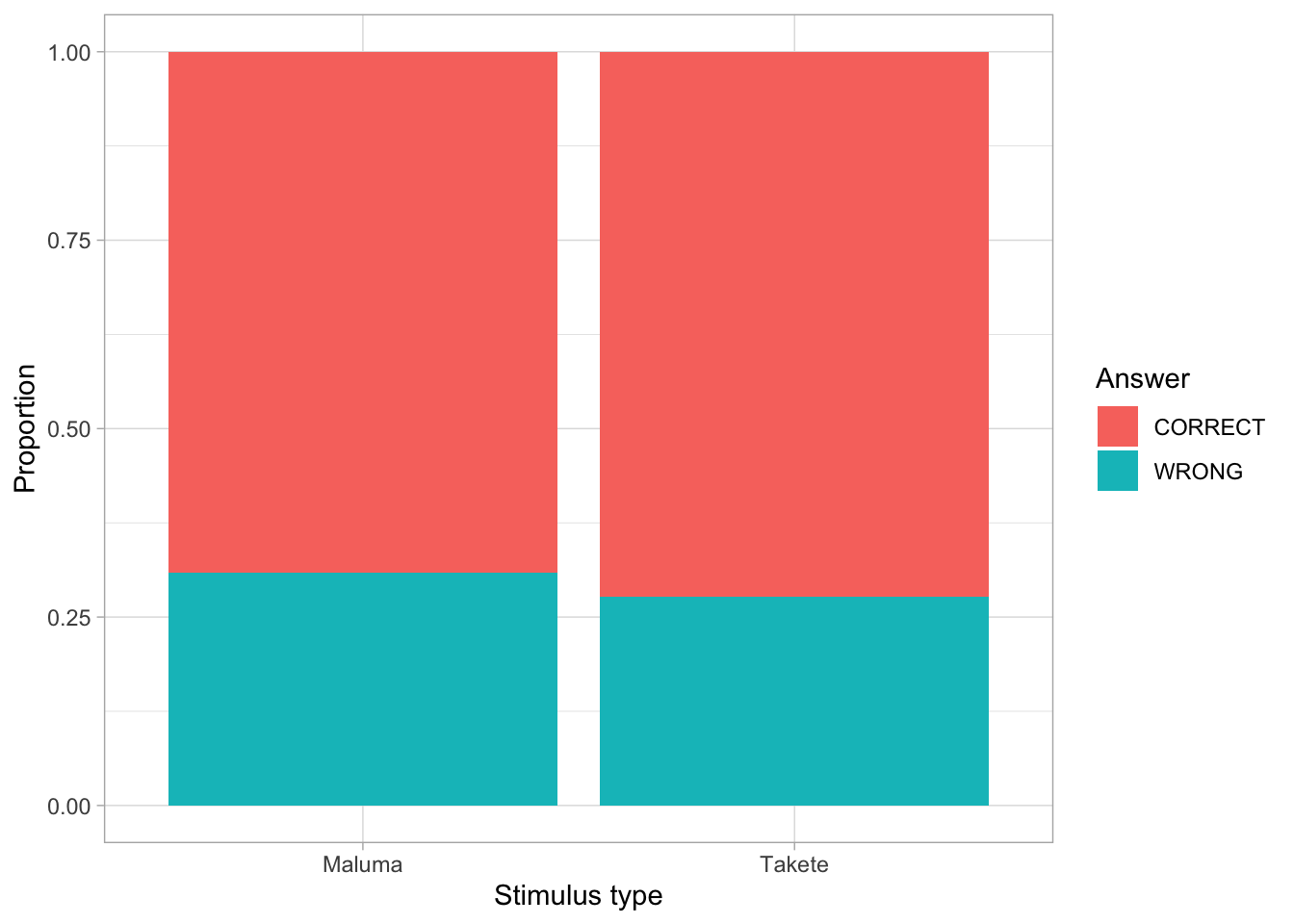
Figure 1: Accuracy by stimulus type.

Modelling accuracy

• We want to model the proportion of correct responses by stimulus type: both types should elicit the same level of accuracy.

• We can use a Bernoulli regression model.

kopper <- kopper |> 
  mutate(
    Answer_f = factor(Answer, levels = c("WRONG", "CORRECT"))
  )
levels(kopper$Answer_f)

[1] "WRONG"   "CORRECT"

Accuracy: Bernoulli regression

kop_bm <- brm(
  Answer_f ~ Tak_Mal_Stim,
  data = kopper,
  family = bernoulli,
  cores = 4,
  seed = 9128,
  file = "cache/kop_bm"
)

Accuracy: model summary

summary(kop_bm)

 Family: bernoulli 
  Links: mu = logit 
Formula: Answer_f ~ Tak_Mal_Stim 
   Data: kopper (Number of observations: 460) 
  Draws: 4 chains, each with iter = 2000; warmup = 1000; thin = 1;
         total post-warmup draws = 4000

Regression Coefficients:
                   Estimate Est.Error l-95% CI u-95% CI Rhat Bulk_ESS Tail_ESS
Intercept              0.81      0.15     0.52     1.11 1.00     3978     2479
Tak_Mal_StimTakete     0.15      0.21    -0.25     0.56 1.00     4026     2442

Draws were sampled using sampling(NUTS). For each parameter, Bulk_ESS
and Tail_ESS are effective sample size measures, and Rhat is the potential
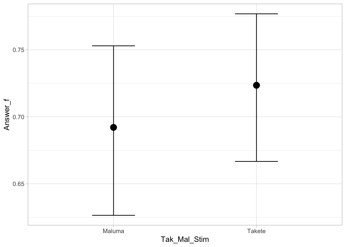
scale reduction factor on split chains (at convergence, Rhat = 1).

Expected predictions of accuracy

Credible intervals of the difference

kop_bm_draws <- as_draws_df(kop_bm)

kop_bm_draws |> 
  summarise(
    `90%` = paste0("[", paste(quantile2(b_Tak_Mal_StimTakete, c(0.05, 0.95)) |> round(2), collapse = ", "), "]"),
    `80%` = paste0("[", paste(quantile2(b_Tak_Mal_StimTakete, c(0.1, 0.9)) |> round(2), collapse = ", "), "]"),
    `70%` = paste0("[", paste(quantile2(b_Tak_Mal_StimTakete, c(0.15, 0.85)) |> round(2), collapse = ", "), "]"),
    `60%` = paste0("[", paste(quantile2(b_Tak_Mal_StimTakete, c(0.2, 0.8)) |> round(2), collapse = ", "), "]"),
    `40%` = paste0("[", paste(quantile2(b_Tak_Mal_StimTakete, c(0.3, 0.7)) |> round(2), collapse = ", "), "]")
  ) |> 
  knitr::kable(align = c("ccccc"))

90%	80%	70%	60%	40%
[-0.18, 0.49]	[-0.11, 0.42]	[-0.06, 0.37]	[-0.02, 0.33]	[0.04, 0.27]

Is there a difference in accuracy by stimulus type?

• According to the model, the difference in log-odds is [-0.25, 0.56] at 95% probability.

• Only at 40% probability we can argue for an increase in log-odds for takete stimuli between 0.04 and 0.27.

• We can’t argue for or against a difference. We just do not know.

References

Chen, Yi-Chuan, Pi-Chun Huang, Andy Woods, and Charles Spence. 2016. “When “Bouba” Equals “Kiki”: Cultural Commonalities and Cultural Differences in Sound-Shape Correspondences.” Scientific Reports 6 (1): 26681. https://doi.org/10.1038/srep26681.

Holland, Morris K., and Michael Wertheimer. 1964. “Some Physiognomic Aspects of Naming, or, Maluma and Takete Revisited.” Perceptual and Motor Skills 19 (1): 111–17. https://doi.org/10.2466/pms.1964.19.1.111.

Köhler, Wolfgang. 1929. Gestalt Psychology. New York: Liveright.

Koppensteiner, Markus, Pia Stephan, and Johannes Paul Michael Jäschke. 2016. “Shaking Takete and Flowing Maluma. Non-Sense Words Are Associated with Motion Patterns.” PLOS ONE 11 (3). https://doi.org/10.1371/journal.pone.0150610.