log_15 <- log(15)
log_15
[1] 2.70805log_15_exp <- exp(log_15)
log_15_exp[1] 15Stefano Coretta
September 12, 2024
Count data is another common type of variable in linguistics. Corpus linguistics in particular usually has count variables, like number of relative clauses or number of direct vs indirect objects to mark the beneficiary.
When modelling count data, the researcher is usually interested in the count themselves. In other cases, they might be interested in the relative counts (proportion) out of a million words or the like (depending on the size of the corpus).
The distribution family for count data is the Poisson family. The Poisson family has only one parameter, \(\lambda\), which is also known as the “rate”. Higher values of \(\lambda\) correspond to greater counts.
Like with Bernoulli models, there is a catch: counts are discrete numeric variables that can only be positive, i.e. they are bounded. Regression models don’t work well with bounded variables (we have seen this for probabilities), so we need to apply a transformation as we did in Bernoulli models.
The transformation used in Poisson models is the (natural) logarithm. The inverse of the logarithm is the exponential function.
For example, we might want to estimate the number of gestures infants produce in a laboratory session. See Cameron 2020 for a description of the study and data variables.
Rows: 1620 Columns: 11
── Column specification ────────────────────────────────────────────────────────
Delimiter: ","
chr (5): dyad, background, task, gesture, pro_rata
dbl (6): months, count_raw, count, ct_raw, ct, id

ℹ Use `spec()` to retrieve the full column specification for this data.
ℹ Specify the column types or set `show_col_types = FALSE` to quiet this message.Let’s estimate the number of gestures (count) depending on the cultural background (background). I recommend creating plots of the data before moving on.
Here’s the model mathematical formula.
\[ \begin{align} \text{N}_i & \sim Poisson(\lambda_i) \\ \ln(\lambda_i) & = \alpha_{\text{B}_i} \end{align} \]
You can read it the first line as:
The number of gestures follows a Poisson distribution with rate \(\lambda_i\).
Counts are a discrete numeric variable, bounded to 0 and positive numbers only. As we have learnt with Bernoulli models, regression models don’t work with bounded variables out of the box. We need to transform counts into a scale that is continuous and unbounded.
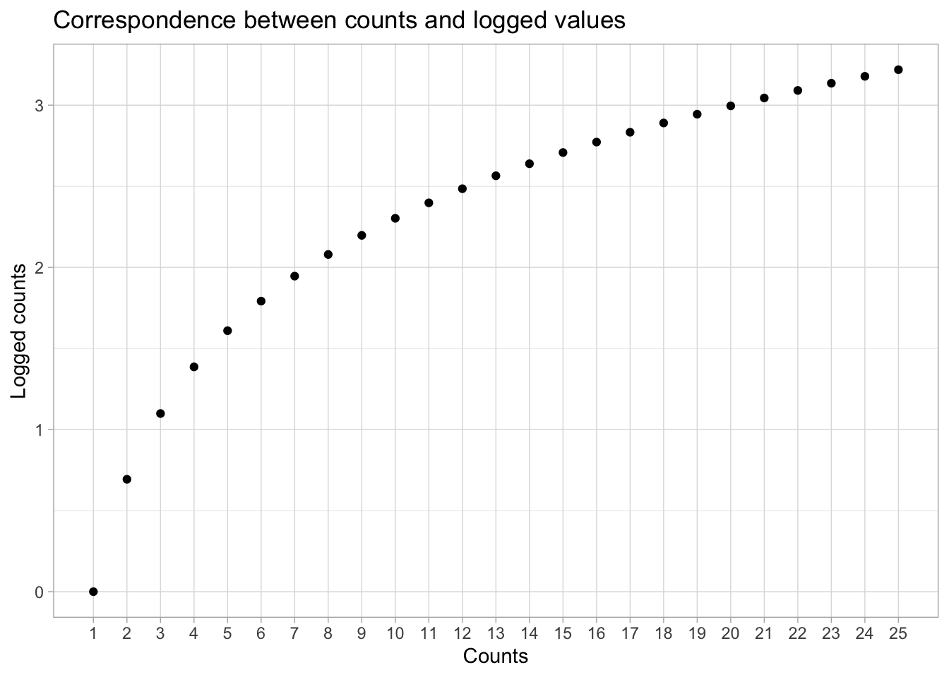
This is where the logarithmic function from the mathematical formula above comes in: the logarithmic function (from “logistic unit”) is a mathematical function that logs numbers.
The plot below shows the correspondence of numbers (on the y-axis) and logged values (on the x-axis), as marked by the black dots. It is helpful to memorise that the log of 1 is 0.

When you fit a regression model with a Poisson distribution, the estimates are log-odds, on the log scale. When you exponentiate the estimates, you go back to the original scale, i.e. counts.
Let’s repeat the model’s mathematical formula here:
\[ \begin{align} \text{N}_i & \sim Poisson(\lambda_i) \\ \ln(\lambda_i) & = \alpha_{\text{B}_i} \end{align} \]
The number of gestures follows a Poisson distribution with rate \(\lambda\).
The log of \(\lambda\) is equal to \(\alpha\) for each background.
In other words, the model estimates \(\lambda\) for each group in background. Here is the code. Remember that to use the indexing approach for categorical predictors (Group) we need to suppress the intercept with the 0 + syntax.
Let’s inspect the model summary (we will get 80% CrIs).
 Family: poisson
  Links: mu = log
Formula: count ~ 0 + background
   Data: gestures (Number of observations: 1599)
  Draws: 4 chains, each with iter = 2000; warmup = 1000; thin = 1;
         total post-warmup draws = 4000

Regression Coefficients:
                  Estimate Est.Error l-80% CI u-80% CI Rhat Bulk_ESS Tail_ESS
backgroundBengali     0.34      0.04     0.30     0.39 1.00     3884     2826
backgroundChinese     0.32      0.04     0.27     0.36 1.00     3863     3086
backgroundEnglish     0.10      0.04     0.04     0.15 1.00     4095     3092

Draws were sampled using sampling(NUTS). For each parameter, Bulk_ESS
and Tail_ESS are effective sample size measures, and Rhat is the potential
scale reduction factor on split chains (at convergence, Rhat = 1).
Based on the model, there is an 80% probability that the logged gesture count is between 0.30 and 0.39 in Bengali infants, 0.27-0.36 in Chinese infants, and 0.04-0.15 in English infants.
It’s easier to understand the results if we convert the logged counts back to counts The quickest way to do this is to get the Regression Coefficients table from the summary with fixef() and mutate the Q columns with exp().
fixef(gest_bm, prob = c(0.1, 0.9)) |>
  # we need to convert the output of fixef() to a tibble to use mutate()
  as_tibble(rownames = "background") |>
  # we plogis() the Q columns and round to the second digit
  mutate(
    Q10 = round(exp(Q10), 2),
    Q90 = round(exp(Q90), 2)
  )
Based on the model and data, there is an 80% probability that the counts of all backgrounds are between 1 and 1.5 gestures. English children do have a slightly lower count of gestures, between 1.05-1.16.
However, a fraction of a gesture does not really make much sense and, linguistically, maybe even a 1 gesture difference will probably be not that relevant. Note that we get fractions of gestures even if we said above that counts are discrete (so there shouldn’t be fractions) because we are converting a continuous scale (logs). This is a quirk of Poisson models and you need to be cautious when comparing estimated counts between groups, like we are doing here.
In sum, we have some evidence that gesture frequency in the different language backgrounds is overall very similar, or that if there are any differences, English infants produce a fraction of a gesture less on average than the other infants.
To conclude this introduction to Poisson models, we can get the predicted counts in the three backgrounds with conditional_effects().