Mutate data

Learn about mutating data using the tidyverse

1 Mutate

library(tidyverse)

glot_status <- readRDS("data/coretta2022/glot_status.rds")

To change existing columns or create new columns, we can use the mutate() function from the dplyr package.

To learn how to use mutate(), we will re-create the status column (let’s call it Status this time) from the Code_ID column in glot_status.

The Code_ID column contains the status of each language in the form aes-STATUS where STATUS is one of not_endangered, threatened, shifting, moribund, nearly_extinct and extinct.

[1] "aes-shifting"       "aes-extinct"        "aes-moribund"      
[4] "aes-nearly_extinct" "aes-threatened"     "aes-not_endangered"

We want to create a new column called Status which has only the STATUS label (without the aes- part). To remove aes- from the Code_ID column we can use the str_remove() function from the stringr package. Check the documentation of ?str_remove to learn which arguments it uses.

glot_status <- glot_status |>
  mutate(
    Status = str_remove(Code_ID, "aes-")
  )

If you check glot_status now you will find that a new column, Status, has been added. This column is a character column (chr).

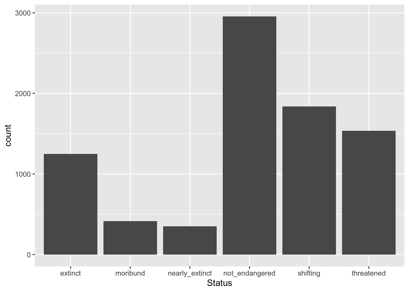
Let’s reproduce the bar chart from above but with all the data from glot_status, using now the Status column.

glot_status |>
  ggplot(aes(x = Status)) +
  geom_bar()

Figure 1: Number of languages by endangerment status (repeated).

But something is not quite right… The order of the levels of Status does not match the order that makes sense (from least to most endangered)! Why?

This is because status (the pre-existing column) is a factor column, rather than a simple character column. What is a factor vector/column?

Factor vector

A factor vector (or column) is a vector that contains a list of values (called levels) from a closed set.

The levels of a factor are ordered alphabetically by default.

A vector/column can be mutated into a factor column with the as.factor() function. In the following code, we change the existing column Status, in other words we overwrite it (this happens automatically, because the Status column already exists, so it is replaced).

glot_status <- glot_status |>
  mutate(
    Status = as.factor(Status)
  )

# read below for an explanation of the dollar disgn $ syntax
levels(glot_status$Status)

[1] "extinct"        "moribund"       "nearly_extinct" "not_endangered"
[5] "shifting"       "threatened"    

The levels() functions returns the levels of a factor column in the order they are stored in the factor: by default the order is alphabetical. But wait, what is that $ in glot_status$Status?

The dollar sign $ a base R way of extracting a single column (in this case Status) from a data frame (glot_status).

The dollar sign `$`

You can use the dollar sign $ to extract a single column from a data frame as a vector.

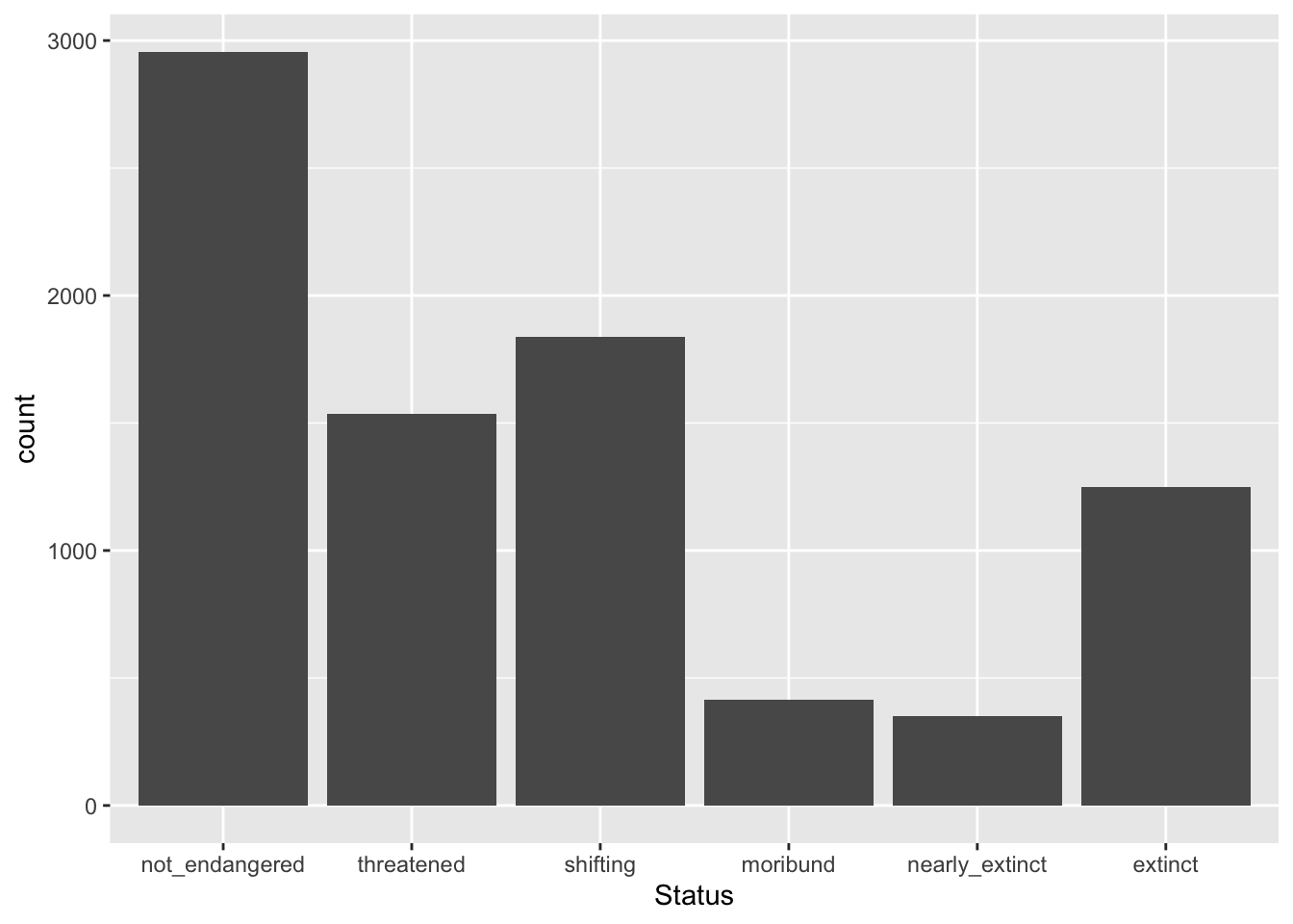
What if we want the levels of Status to be ordered in a more logical manner: not_endangered, threatened, shifting, moribund, nearly_extinct and extinct? Easy! We can use the factor() function instead of as.factor() and specify the levels and their order.

glot_status <- glot_status |>
  mutate(
    Status = factor(Status, levels = c("not_endangered", "threatened", "shifting", "moribund", "nearly_extinct", "extinct"))
  )

levels(glot_status$Status)

[1] "not_endangered" "threatened"     "shifting"       "moribund"      
[5] "nearly_extinct" "extinct"       

You see that now the order of the levels returned by levels() is the one we specified.

Transforming character columns to vector columns is helpful to specify a particular order of the levels which can then be used when plotting.

glot_status |>
  ggplot(aes(x = Status)) +
  geom_bar()

Figure 2: Number of languages by endangerment status (repeated).