mald <- readRDS("data/tucker2019/mald_1_1.rds")Regression models: interactions
1 Introduction
Regression models can include both numeric and categorical predictors. Numeric predictors can be included in regression models directly, while categorical predictors have to be coded numerically (regression models can only work with numeric stuff). Coding of categorical predictors is done automatically by R when you include categorical predictors. There are two main type of coding approaches: contrasts (the default) and indexing.
Indexing of categorical predictors is helpful when including multiple predictors in a regression model. So far, we only had one predictor per model. In this tutorial you will learn how to include and interpret regression models with multiple predictors.
We will also explore the concept of predictor interactions. In brief, an interaction between two predictors allows the model to adjust the effect of one predictor depending on the value/level of another, and vice versa. To illustrate interactions, we will use the Massive Auditory Lexical Decision data, MALD.
2 The data: Massive Auditory Lexical Decision (MALD)
Let’s read the data. They are in an .rds file, so we need readRDS().
We will focus on reaction times (RT) and the phonetic Levinstein distance (PhonLev). Specifically, we will investigate the effect of the phonetic distance on RTs depending on the lexical status of the the word heard by participants (i.e. where the word was a real word or a nonce word, IsWord).
mald |>
  ggplot(aes(PhonLev, RT)) +
  geom_point(alpha = 0.1) +
  geom_smooth(aes(colour = IsWord, fill = IsWord), method = "lm", formula = "y ~ x")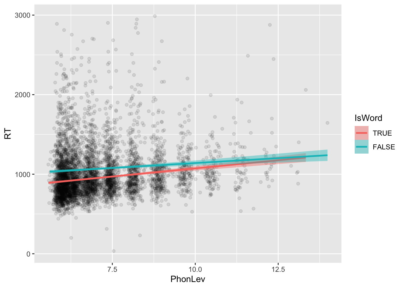
The scatter plot above includes two regression lines: one for real words (IsWord = TRUE) and one for nonce words (IsWord = FALSE). Generally, increasing phonetic distance corresponds to increasing RTs (i.e. slower responses). This positive relationship also differs somewhat depending on the word lexical status. Try and find more patterns in the plot and make a mental record. You will be able to compare your intuitions with the regression results later.
3 Regression with two predictors: IsWord and PhoneLev
We start by fitting a regression model with logged RTs as the outcome variable and a Gaussian distribution as the probability distribution of RTs. We include IsWord and PhonLev. IsWord will be coded with indexing (rather than the default contrasts).
\[ \begin{align} log(RT)_i & \sim Gaussian(\mu_i, \sigma)\\ \mu_i & = \alpha_{\text{W}[i]} + \beta \cdot \text{PL}_i \end{align} \]
- \(\alpha_{\text{W}[i]}\) is the mean RT value depending on
IsWord. - \(\beta\) is the change in RT for each unit increase of phonetic distance (
PhonLev).
The mathematical formula corresponds to the R formula RT_log ~ 0 + IsWord + PhonLev. Let’s fit the regression model with this formula now.
mald_bm_1 <- brm(
  RT_log ~ 0 + IsWord + PhonLev,
  family = gaussian,
  data = mald,
  seed = 9284,
  cores = 4,
  file = "cache/regression-interactions_mald_bm_1"
)
Let’s check the summary.
summary(mald_bm_1, prob = 0.8) Family: gaussian
Links: mu = identity; sigma = identity
Formula: RT_log ~ 0 + IsWord + PhonLev
Data: mald (Number of observations: 5000)
Draws: 4 chains, each with iter = 2000; warmup = 1000; thin = 1;
total post-warmup draws = 4000
Regression Coefficients:
Estimate Est.Error l-80% CI u-80% CI Rhat Bulk_ESS Tail_ESS
IsWordTRUE 6.58 0.02 6.55 6.61 1.01 1104 1477
IsWordFALSE 6.69 0.02 6.66 6.72 1.00 1095 1401
PhonLev 0.03 0.00 0.03 0.04 1.00 1115 1441
Further Distributional Parameters:
Estimate Est.Error l-80% CI u-80% CI Rhat Bulk_ESS Tail_ESS
sigma 0.27 0.00 0.27 0.27 1.00 1670 1318
Draws were sampled using sampling(NUTS). For each parameter, Bulk_ESS
and Tail_ESS are effective sample size measures, and Rhat is the potential
scale reduction factor on split chains (at convergence, Rhat = 1).IsWordTRUEis the estimated logged RT whenIsWordisTRUE: at 80% probability, it is between 6.55 and 6.61 logged milliseconds, i.e. 699 and 742 ms (exp(6.55)andexp(6.61)).IsWordFALSEis the estimated logged RT whenIsWordisFALSE: at 80% probability, it is between 6.66 and 6.72 logged milliseconds, i.e. 781 and 829 ms (exp(6.66)andexp(6.72)).PhonLevis the estimated change in logged RTs for each unit increase ofPhonLev: at 80% probability, whenPhonLevincreases by 1, logged RTs increase by 0.03 to 0.04 logged ms.
Make sure you understand how to interpret the coefficients! A lot of learners of statistics get easily confused by this and when model start to become more complex, things will be even more difficult to disentangle.
4 Centring numeric predictors
In mald_bm_1, the coefficients for IsWord are the estimated logged RT when PhonLev is 0 and the coefficient for PhonLev is approximately the average change in logged RTs across the two IsWord conditions! This is a very important aspect of regression models with multiple predictors.
Let’s focus on the when PhonLev is 0 part. In some cases, 0 for numeric predictors is meaningful (for example, if you are counting hand gestures of infants, a count of 0 makes sense, it just means that the infant did not produce any gesture), but in other cases 0 does not make sense: a typical example is duration or length, like segment duration. A segment, like a vowel, can’t be 0 ms long: that would mean there is no vowel!
In those cases where 0 is not meaningful for a numeric predictor, a typical approach is to centre that predictor.
Centring is a transformation by which you subtract the mean value from all of the observations of the numeric predictor. Check the code below if it’s not immediately clear how it works. The mean RT value in the data is about 7. Mathematically, the model is:
\[ \begin{align} log(RT)_i & \sim Gaussian(\mu_i, \sigma)\\ \mu_i & = \alpha_{\text{W}[i]} + \beta \cdot (\text{PL}_i - \bar{\text{PL}}) \end{align} \]
mald <- mald |>
  mutate(
    # centre variable
    PhonLev_c = PhonLev - mean(PhonLev)
  )
Let’s plot both PhonLev and PhonLev_c to see what happened.
mald |>
  ggplot(aes(PhonLev)) +
  geom_density() +
  geom_rug(alpha = 0.1)
mald |>
  ggplot(aes(PhonLev_c)) +
  geom_density() +
  geom_rug(alpha = 0.1)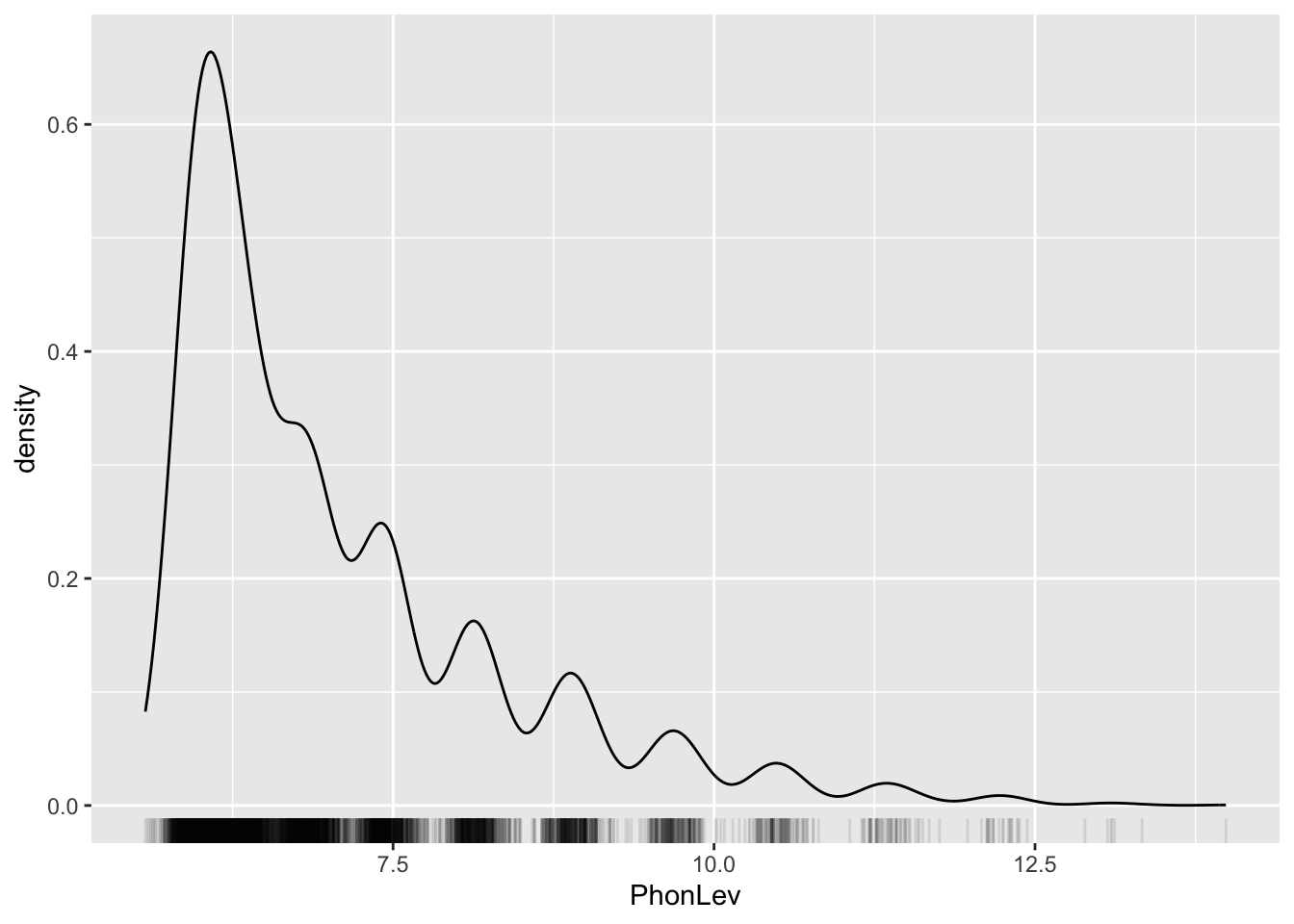

You will see that the shape of the density distribution is unchanged, but the values on the x-axis are now different. If you compare the two plots, you will notice that in the centred version 0 lies at about the same spot that corresponds to 7 in the non-centred version. This makes sense, since centring transforms the data so that the mean (here, 7) becomes 0. The other values can be thought of as differences from the mean.
If you include the centred PhonLev_c in the model, now the estimated logged RT for IsWord will be when PhonLev is at its mean. Why? Because they will be the estimates when PhonLev_c is 0, which corresponds to the mean PhonLev because of the centring transformation!
Let’s fit the model and check the summary.
mald_bm_2 <- brm(
  RT_log ~ 0 + IsWord + PhonLev_c,
  family = gaussian,
  data = mald,
  seed = 9284,
  cores = 4,
  file = "cache/regression-interactions_mald_bm_2"
)

summary(mald_bm_2, prob = 0.8)
Family: gaussian
Links: mu = identity; sigma = identity
Formula: RT_log ~ 0 + IsWord + PhonLev_c
Data: mald (Number of observations: 5000)
Draws: 4 chains, each with iter = 2000; warmup = 1000; thin = 1;
total post-warmup draws = 4000
Regression Coefficients:
Estimate Est.Error l-80% CI u-80% CI Rhat Bulk_ESS Tail_ESS
IsWordTRUE 6.82 0.01 6.82 6.83 1.00 4106 3124
IsWordFALSE 6.93 0.01 6.93 6.94 1.00 4152 2987
PhonLev_c 0.03 0.00 0.03 0.04 1.00 5878 3035
Further Distributional Parameters:
Estimate Est.Error l-80% CI u-80% CI Rhat Bulk_ESS Tail_ESS
sigma 0.27 0.00 0.27 0.27 1.00 3361 2808
Draws were sampled using sampling(NUTS). For each parameter, Bulk_ESS
and Tail_ESS are effective sample size measures, and Rhat is the potential
scale reduction factor on split chains (at convergence, Rhat = 1).The estimates of the coefficients IsWordTRUE and IsWordFALSE have changed: they are now somewhat higher than the estimates in mald_bm_1. This is because increasing phonetic distance increases RTs too: this means that estimated RTs when PhonLev is 0 will be lower than estimated RTs when PhonLev is at the mean of 7 (i.e. when PhonLev_c is at 0).
You will also notice, however, that the estimated effect of PhonLev_c is the same as the estimated effect of PhonLev. This is because centring is a linear transformation: all values are changed in the same way and this does not affect the change in RTs for each unit increase of phonetic distance.
Let’s plot the predictions from this model with conditional_effects().
conditional_effects(mald_bm_2, "PhonLev_c:IsWord")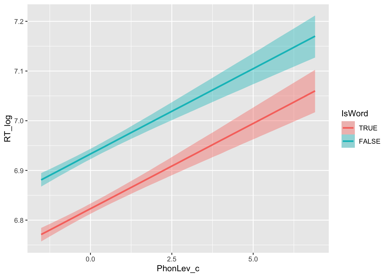
We can tell that on average the RT for nonce words (IsWord = FALSE) are longer than those for real words (IsWord = TRUE). Moreover, increasing phonetic distance corresponds to increasing RT values: the more unique a word is, the longer it takes to make a lexical decision.
But you will also notice something: the estimated regression lines in the two IsWord conditions have exactly the same slope, meaning that the effect of phonetic distance is the same in both conditions.
This doesn’t seem to be right when comparing this with the plot we made above, using the raw data. While comparing raw and estimated data is not always straightforward, here we are missing an important tool in our model that creates the discrepancy: predictor interactions (or simply, interactions).
5 Interactions: categorical * numeric
The model mald_bm_2 estimates the same effect of PhonLev_c in both IsWord conditions because we didn’t include an interaction term: interaction terms allow the model to adjust the effects of each of the predictors in the interaction based on the value of the other predictors in the interaction.
Let’s look at the mathematical specification of a model with an interaction.
\[ \begin{align} log(RT)_i & \sim Gaussian(\mu_i, \sigma)\\ \mu_i & = \alpha_{\text{W}[i]} + \beta_{\text{W}[i]} \cdot (\text{PL}_i - \bar{\text{PL}}) \end{align} \]
The new part is the interaction term: \(\beta_{\text{W}[i]} \cdot (\text{PL}_i - \bar{\text{PL}})\): now \(\beta\) is estimated for IsWord = TRUE and IsWord = FALSE.
Interaction terms in R are specified by using a colon: :: IsWord:PhonLev_c. See the following code.
mald_bm_3 <- brm(
  RT_log ~ 0 + IsWord + IsWord:PhonLev_c,
  family = gaussian,
  data = mald,
  seed = 9284,
  cores = 4,
  file = "cache/regression-interactions_mald_bm_3"
)
0 +suppresses the intercept (we need this to use to indexing approach instead of the default contrasts approach).IsWordcorresponds to \(\alpha_{\text{W}[i]}\) above.IsWord:PhonLev_ccorresponds to \(\beta_{\text{W}[i]} \cdot (\text{PL}_i - \bar{\text{PL}})\).
summary(mald_bm_3, prob = 0.8) Family: gaussian
Links: mu = identity; sigma = identity
Formula: RT_log ~ 0 + IsWord + IsWord:PhonLev_c
Data: mald (Number of observations: 5000)
Draws: 4 chains, each with iter = 2000; warmup = 1000; thin = 1;
total post-warmup draws = 4000
Regression Coefficients:
Estimate Est.Error l-80% CI u-80% CI Rhat Bulk_ESS
IsWordTRUE 6.82 0.01 6.82 6.83 1.00 5106
IsWordFALSE 6.93 0.01 6.93 6.94 1.00 4753
IsWordTRUE:PhonLev_c 0.04 0.00 0.04 0.05 1.00 5624
IsWordFALSE:PhonLev_c 0.03 0.00 0.02 0.03 1.00 5295
Tail_ESS
IsWordTRUE 2696
IsWordFALSE 2665
IsWordTRUE:PhonLev_c 3391
IsWordFALSE:PhonLev_c 3013
Further Distributional Parameters:
Estimate Est.Error l-80% CI u-80% CI Rhat Bulk_ESS Tail_ESS
sigma 0.27 0.00 0.27 0.27 1.00 4005 2810
Draws were sampled using sampling(NUTS). For each parameter, Bulk_ESS
and Tail_ESS are effective sample size measures, and Rhat is the potential
scale reduction factor on split chains (at convergence, Rhat = 1).IsWordTRUE: the estimated logged RT whenIsWordisTRUEandPhonLev_cis 0.IsWordFALSE: the estimated logged RT whenIsWordisFALSEandPhonLev_cis 0.IsWordTRUE:PhonLev_c: the estimated change in RT for each unit increase ofPhonLev_cwhenIsWordisTRUE.IsWordFALSE:PhonLev_c: the estimated change in RT for each unit increase ofPhonLev_cwhenIsWordisFALSE.
Let’s transform the estimates to milliseconds (for IsWord) and percentage change (for the interaction with PhoneLev_c).
round(exp(c(6.82, 6.83)))[1] 916 925round(exp(c(6.93, 6.94)))[1] 1022 1033round(exp(c(0.04, 0.05)), 2)[1] 1.04 1.05round(exp(c(0.02, 0.03)), 2)[1] 1.02 1.03You can report the results of this model like so:
We fitted a Bayesian regression with logged reaction times (RTs) as the outcome variable and a Gaussian distribution as the distribution of the outcome. As predictors, we included lexical status (
IsWord, categorical, coded asTRUEfor real words andFALSEfor nonce words) and an interaction between lexical status and phonetic distance (PhonLev_c, numeric centred). The categorical predictor of lexical status was coded using indexing by suppressing the model intercept with the0 +syntax. See @tab-bm-3 for the coefficient estimates.Based on the model, at mean phonetic distance, RTs are between 916 and 925 ms when the word is a real word and between 1022 and 1033 ms when the word is a nonce word, at 80% confidence. For each unit increase of phonetic distance, RTs increase by 4-5% with real words and by 2-3% with nonce words, at 80% probability.
And now, the visual proof that including an interaction allows the model to adjust the effect of phonetic distance.
conditional_effects(mald_bm_3, "PhonLev_c:IsWord")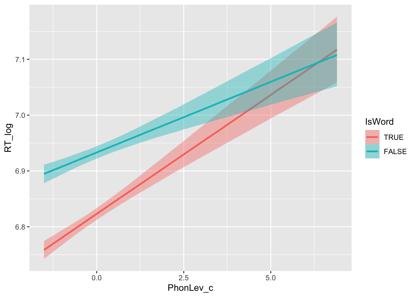
Note that including an interaction term is important whenever you want to know if indeed the effect of a predictor depends on the value of other predictors. Furthermore, including an interaction term when the effect does not differ between values of other predictors is not an issue for model fitting: you will just get similar estimated effects for all the values of the other predictors.
6 Wrangling draws of numeric predictors
Let’s inspect the MCMC draws.
mald_3_draws <- as_draws_df(mald_bm_3)

mald_3_draws
Nothing out of the ordinary: the drawn values for our regression coefficients are in the columns that start with b_ (and there is also sigma of course).
Most times it is helpful to get estimates not only when you increase your numeric predictor by 1, but also when you increase it further. For example, in our data we see that at lower phonetic distance values, the estimated RTs are quite different depending on IsWord. But with increasing phonetic distance, the difference in RTs between the two IsWord conditions becomes smaller and smaller.
So now we can ask the question: what is the estimated difference in RTs between IsWord = TRUE and IsWord = FALSE when phonetic distance is 12?
Since PhoneLev_c is centred, if we want to get phonetic distance 12 we need to find the corresponding PhonLev_c values. Since the mean of PhonLev is about 7, then 12 corresponds to 5 in PhonLev_c (7 + 5 = 12).
To get the estimated RT value in real and nonce words when the phonetic distance is 12, we just add the coefficient of PhonLev_c multiplied by 5. This is because the estimate is for each unit increase of phonetic distance, but we want to get the estimated RT when phonetic distance increases by 5 from the mean (i.e. when it is 12). Look at the code below.
Since the interaction terms have : in their names and : is a special symbol in R, you need to “protect” the name by surrounding it between back ticks `.
mald_3_preds_5 <- mald_3_draws |>
  mutate(
    word_5 = b_IsWordTRUE + (5 * `b_IsWordTRUE:PhonLev_c`),
    non_word_5 = b_IsWordFALSE + (5 * `b_IsWordFALSE:PhonLev_c`),
  )

mald_3_preds_5 |>
  select(word_5:non_word_5)
Warning: Dropping 'draws_df' class as required metadata was removed.Now that we have the draws of logged RT values for real and nonce words when phonetic distance is 12, we can take the difference between the two and calculate the 80% CrI of that difference. We want the difference in milliseconds, rather than logged milliseconds, so we exponentiate the logged values before taking the difference.
library(posterior)This is posterior version 1.6.0
Attaching package: 'posterior'The following objects are masked from 'package:stats':
mad, sd, varThe following objects are masked from 'package:base':
%in%, matchmald_3_preds_5 |>
mutate(
word_nonword_5 = exp(non_word_5) - exp(word_5)
) |>
summarise(
lo_80 = quantile2(word_nonword_5, 0.1),
hi_80 = quantile2(word_nonword_5, 0.9),
)You could add the report above:
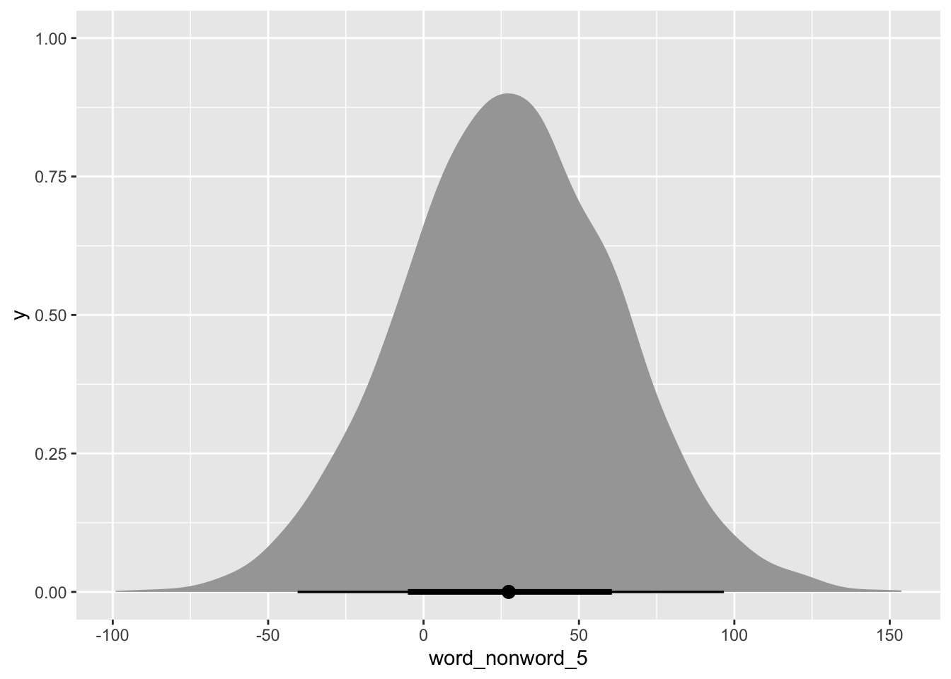
At 80% confidence, when the phonetic distance is 12, RTs when the word is a nonce word are -17 ms shorter to 74 ms longer than when the word is a real word.
We can also plot the posterior draws of the difference as we would with any posterior draws.
library(ggdist)
Attaching package: 'ggdist'The following objects are masked from 'package:brms':
dstudent_t, pstudent_t, qstudent_t, rstudent_tmald_3_preds_5 |>
mutate(
word_nonword_5 = exp(non_word_5) - exp(word_5)
) |>
ggplot(aes(word_nonword_5)) +
stat_halfeye()